How to Create a Dropdown List in Google Sheets
Google Sheets is available online as a great tool that allows many people to create, edit, read, and make necessary changes concurrently. While this is great, some data inputted by other people may cause some confusion.

Nov 21 2019●6 min read
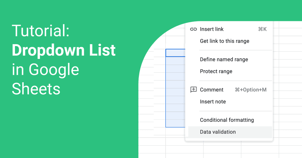
Hence, there is a need to control the information options available to users in such cases. The dropdown validation list is perfect for this, as it ensures that only the information that is needed is entered.
With it, any spreadsheet should be created conveniently and used in the form of a questionnaire, a marking guide, and so much more!
Follow these guidelines to get started on creating a dropdown in Google Sheets.
Can You Make A Drop Down Menu In Google Sheets?
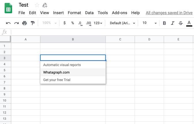
A dropdown list is generally known as a data validation method that can be applied to a specific number of cells on a particular spreadsheet to ensure that the information entered on the sheet is not different from what is expected.
You should be able to create, edit, and modify a dropdown on all devices that work with Android, Linux, Windows, Chrome OS, or macOS. However, with an iOS device, you might be able to view only and use those Google Sheets drop-down list.
How Do You Create A Drop Down?
The foremost step, of course, is to open files relating to Google Sheets dropdown menu on your device. Then, follow these steps listed below:
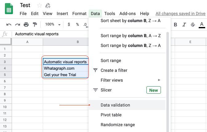
Highlight the cells you want to have your dropdown menu appear in by dragging your mouse across them or using the shift+arrow command. You could select as many cells as you want.
At the top menu, click on "Data" and select "Data Validation". Alternatively, you could right-click the highlighted cells and select "Data Validation".
 |  |  |
What Is Data Validation In Google Sheets?
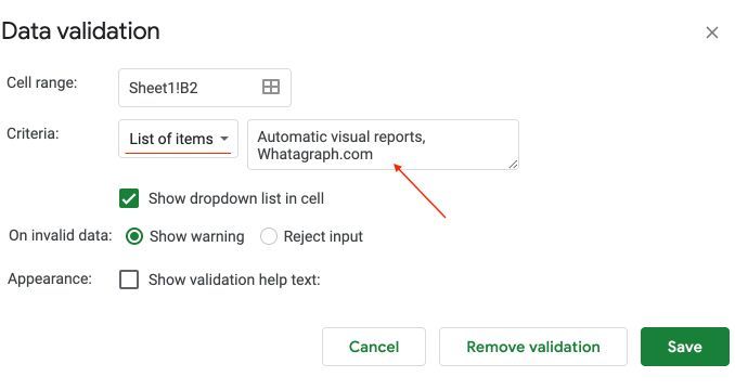
In the Data Validation interface, you would see some options you can modify to design your dropdown list:
- "Cell Range" is for selecting the cells you want your dropdown lists to appear in on that file. If you have pre-selected them with your mouse or keyboard, the cell numbers would already be stated.
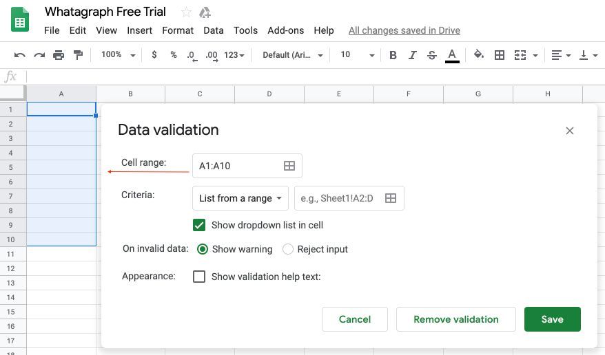 |
- Next is "Criteria", which contains a dropdown menu of the specific kinds of data you want to be inputted on your sheet. You could choose "List of Items", "Date", "Numbers", and so on. Below these options is an input box for your type in the exact words, numbers, formulas, or items you want people to enter in the cell ranges you selected.
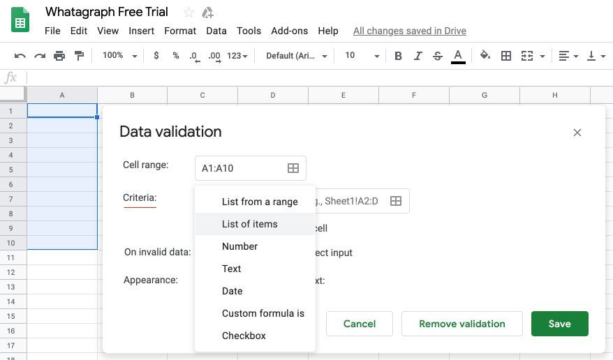 |
- "Criteria" is more or less divided into six distinct parts: List, Checkbox, Text/Email/URL validity, Date, Number, and Custom Data.
How To Make A Drop Down List In Google Sheets
For lists, you can either select "List of Items" or "List from a Range".
"List of Items" allows you to input a list of predetermined data items, which could be numbers or texts. You would input them in the box below and separate each with a comma.
If you choose a criterion that provides a dropdown list, you would be required to select if you want the dropdown to be visible to users or if users are allowed to type in data that would then be validated. Either of these can be specified by selecting the "Show dropdown list in cell" or not.
Next is "Appearance", which allows you to give users a guideline on what kind of data is expected to be inputted in the selected cell range.
After this, you also get to determine if the wrong data should be rejected or not with the options provided in "On invalid data". If you select "Show Warning", users would be allowed to enter invalid data into the sheet, but it would be marked. This status is great for collecting new data that is not included in your configured list. With "Reject Input", invalid entries will not be accepted at all.
After you've satisfactorily configured your dropdown list in Google Sheets, click "Save".
How Do You Color Code A Drop Down List In Google Sheets?
One interesting thing is that it does not have to end there. Colors are tools that are useful in data collection, as they help sort answers quicker. They could also engage users, especially children. If you plan to use your Google Sheet as a questionnaire for kids, or you simply what to make sorting data easier for yourself, you might consider color-coding your dropdown list.
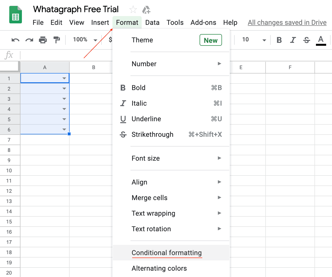
By using the "Conditional Formatting" option, you would be able to achieve this. Here's what you should do:
- Highlight the dropdown list cells you want to color code;
- Select "Conditional Formatting";
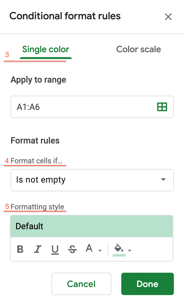
- Conditional Formatting had two interfaces, "Single Color" and "Color Scale". In the "Single Color" interface, the cells you have highlighted would appear in the "Apply to Range" input box (you could also input the cell range here instead of highlighting them);
- The next option is "Format cell if...". This option allows you to select the condition in which you want your pre-selected range to adopt a color. It is similar to "Criteria" in "Data Validation";
- Next is the "Formatting Style" that allows you to choose a color;
- With "Custom", you could do some extra formatting;
- When you are done, "Save/Add New"
- You can apply the same technique in the "Color Scale" interface. "Color Scale" is great for numbers.
 |  |
Conclusion
Now that you are now well informed about how to create a drop-down list in Google Sheets try it out and fine-tune it to your preference! If you want to learn more tips and tricks, check this Google Sheets guide out. After some practice, you should be able to create a drop-down list in google sheets.

WRITTEN BY
Indrė Jankutė-CarmaciuIndrė is a copywriter at Whatagraph with extensive experience in search engine optimization and public relations. She holds a degree in International Relations, while her professional background includes different marketing and advertising niches. She manages to merge marketing strategy and public speaking while educating readers on how to automate their businesses.


